Until 2014, CNN architectures had a standard design:

1. Stacked convolutional layers with ReLU activations
2. Optionally followed by contrast normalization and max-pooling and dropouts to address the problem of overfitting
3. Followed by one or more fully connected layers at the end

Variants of this design were prevalent in the image classification literature and had yielded the best results on MNIST and CIFAR10/100 datasets. On the ImageNet classification challenge dataset the recent trend had been to increase the number of layers (depth) and number of units at each level (width) blindly. Despite trends, taking inspiration and guidance from the theoretical work done by Arora et al. GoogLeNet takes a slightly different route for its architectural design.

Major Drawbacks of Design Trend for a Bigger Size

1. A large number of parameters - which makes the enlarged network more prone to overfitting, especially if the number of labeled examples in the training set is limited.

2. Increased use of computational resources - any uniform increase in the number of units in two consecutive convolutional layers, results in a quadratic increase in computation. The efficient distribution of computing resources is always preferred to an indiscriminate increase in size since practically the computational budget is always finite.

The Approach

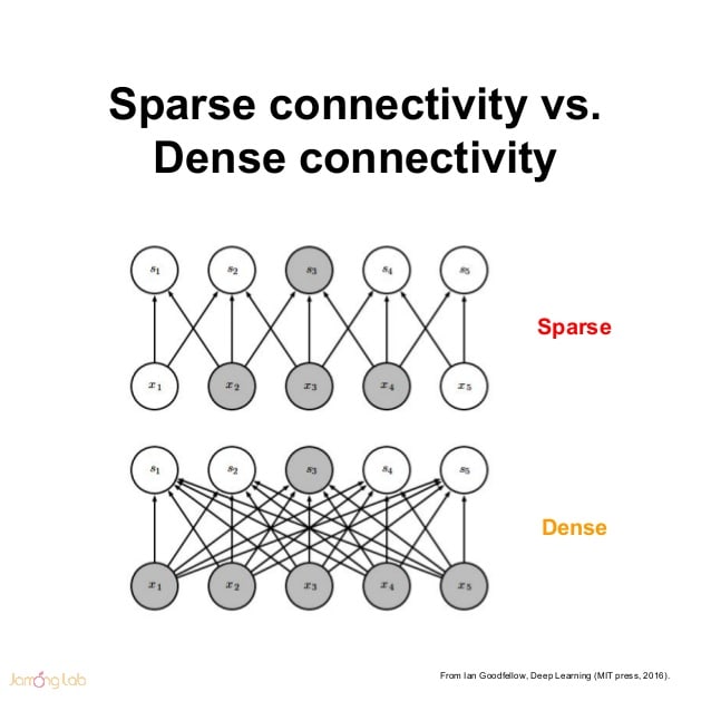
The main result of a theoretical study performed by Aurora et al. states that if the probability distribution of the dataset is representable by a large, very sparse deep neural network, then the optimal network topology can be constructed layer-by-layer by analyzing the correlation statistics of the activations of the last layer and clustering neurons with highly correlated outputs. The statement resonates with the well known Hebbian principle – neurons that fire together, wire together.
In short, the approach as suggested by the theory was to build a non-uniform sparsely connected architecture that make use of the extra sparsity, even at the filter level. But since AlexNet, to better optimize parallel computing, convolutions were implemented as collections of dense connections to the patches in the earlier layer.

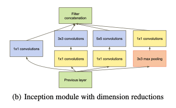
So based on suggestions by Çatalyürek et al. to obtain SOTA performance for sparse matrix multiplication, authors clustered sparse matrices into relatively dense submatrices, thus approximating an optimal local sparse structure in a CNN layer (Inception module) and repeating it spatially all over.

Architectural Details

One big problem with this stacked inception module is that even a modest number of 5×5 convolutions would be prohibitively expensive on top of a convolutional layer with numerous filters. This problem becomes even more pronounced once pooling units are added. Even while the architecture might cover the optimal sparse structure, it would do that very inefficiently; the merging of the output of the pooling layer with the outputs of convolutional layers would definitely lead to a computational blow up within a few stages.

Thus, authors borrowed Network-in-Network architecture which was proposed by Lin et al. to increase the representational power of neural networks. It can be viewed as an additional 1 × 1 convolutional layer followed typically by the ReLU activation. Authors applied it in forms of

• dimension reductions - 1×1 convolutions used for computing reductions before the expensive 3×3 and 5×5 convolutions
• projections - 1×1 convolutions used for shielding a large number of input filters of the last stage to the next after max-pooling

wherever the computational requirements would increase too much (computational bottlenecks). This allows for not just increasing the depth, but also the width of our networks without a significant performance penalty.

Authors also added auxiliary classifiers, taking the form of smaller convolutional networks on top of the output of the Inception (4a) and (4d) modules, expecting to

1. encourage discrimination in the lower stages in the classifier
2. increase the gradient signal that gets propagated back
3. provide additional regularization. 

During training, their loss gets added to the total loss of the network with a discount weight of 0.3. At inference time, these auxiliary networks were discarded.

The exact structure of these auxiliary classifiers is as follows:

• An average pooling layer with 5×5 filter size and stride 3, resulting in a 4×4×512 output for the (4a), and 4×4×528 for the (4d) stage.
• A 1×1 convolution with 128 filters for dimension reduction and rectified linear activation.
• A fully connected layer with 1024 units and rectified linear activation.
• A dropout layer with a 70% ratio of dropped outputs.
• A linear layer with softmax loss as the classifier (predicting the same 1000 classes as the main classifier, but removed at inference time).

The complete architecture of GoogLeNet:

Training

It was trained using the DistBelief distributed machine learning system.

Image Transformations
Photometric distortions by Andrew Howard were useful to combat overfitting to some extent

Optimizer
SGD with Nesterov accelerated gradient of 0.9 momentum

Learning Rate Manager
Decreasing the learning rate by 4% every 8 epochs

No. of Layers
22

Results

Classification

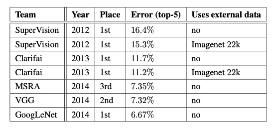
Authors adopted a set of techniques during testing to obtain a higher performance:

1. Independently trained 7 versions of the same GoogLeNet model, and performed ensemble prediction with them. They only differ in sampling methodologies and the random order in which they see input images.

2. Adopted a more aggressive cropping approach than that of AlexNet. Specifically, authors resized the images to 4 scales where the shorter dimension (height or width) was 256, 288, 320 and 352 respectively, taking the left, center, and the right square of these resized images (if portrait images, take the top, center and bottom squares). For each square, they then took the 4 corners and the center 224×224 crop as well as the square resized to 224×224, and their mirrored versions. This results in 4×3×6×2 = 144 crops per image.

3. The softmax probabilities are averaged over multiple crops and overall the individual classifiers to obtain the final prediction.

GoogleNet ranked first.

Object Detection

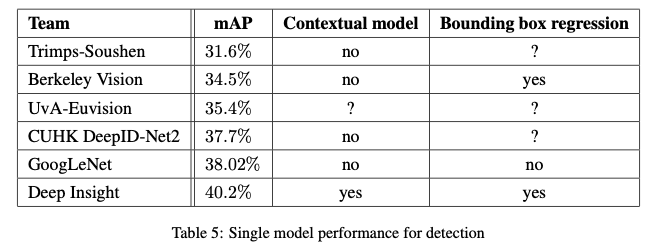
The approach by GoogLeNet for detection was similar to the R-CNN proposed by Girshick et al., but augmented with the Inception model as the region classifier.
Note: R-CNN decomposes the overall detection problem into two subproblems: to first utilize low-level cues such as color and superpixel consistency for potential object proposals in a category-agnostic fashion, and to then use CNN classifiers to identify object categories at those locations.

The region proposal step is improved here by combining the Selective Search approach with multi-box predictions for higher object bounding box recall. To cut down the number of false positives, the superpixel size was increased two folds, improving the mAP (mean average precision) metric by 1% for the single model case. Contrary to R-CNN, they did not use bounding box regression and localization data for pretraining.

Finally, they use an ensemble of 6 CNNs when classifying each region which improves results from 40% to 43.9% mAP, drawing them to the top.

Remarks

GoogLeNet's success promised a future towards creating sparser and more refined structures for CNN architectures. It also conveyed a strong message on consideration of a model's power and memory use efficiency while designing a new architecture. Similar to VGGNet, GoogLeNet also reinstated that going deeper and wider was indeed the right direction to improve accuracy.