One of the running themes throughout this series has been the idea of making large, complex problems, which at first may seem super intimidating, feel so much more approachable. If we want to get really meta about it, that’s what the mission of this entire series is, really: to make the complexities of computer science seem fun, friendly, and thus, far more approachable!

But even on a microcosmic level, we’ve done this in many ways for each topic that we’ve covered. We dissected complex data structures like stacks and queues and chiseled them down into their smaller moving parts. We worked our way up to complex algorithms by understanding and slowly and systematically building upon the little pieces that these larger algorithms are all based upon.

Well, guess what? This technique is far from unique. In fact, it’s probably one of the most commonly-used approaches to problem solving in the world of computer science! Breaking down a problem into smaller, more bite-sized parts is something that computer scientists and programmers alike have been doing for decades. This method is tried, tested, and repeatedly been proven to be true. It’s so commonplace that it has its own name: dynamic programming. Even if you’ve never heard of this term before, there’s a good chance that you’ve either used dynamic programming or are already somewhat familiar with its core concepts.

For our purposes, dynamic programming is particularly useful to understand in the context of algorithm design. We’ve dealt with a whole lot of algorithms over the course of this series, from sorting algorithms, to traversal algorithms, to path-finding algorithms. However, we haven’t really talked about the ways that these algorithms are constructed. Not to worry – all of that changes today. It’s time for us to put our designer hats on for a change, and dive into the delicate intricacies of designing algorithms using the principles of dynamic programming.

Let’s get to it!

Paradigms of algorithm design

The term dynamic programming (abbreviated as “DP”) has a reputation for sounding for more intimidating than what it actually is. I think a large part of this has to do with its name, which – to me at least – sounds really complicated. But we’ll come back to the name a bit later. Let’s start with a definition in order to try to wrap our heads around what on earth “dynamic programming means.

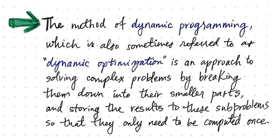
A helpful way to think about dynamic programming is by remembering that it is always tied to optimization , which is the idea that an algorithm should always choose the best possible element at any given time, regardless of whether it is sorting, searching, traversing through a structure, or finding a path. Because dynamic programming is rooted in optimization, this term is interchangeable with the term dynamic optimization.

But how exactly is dynamic programming or dynamic optimization connected to optimizing an algorithm? In other words, what does this form of algorithm design do to optimize an algorithm?

Well, at the end of the day, a dynamic programming algorithm solves a complex problem by breaking it down into its smaller parts. After a DP algorithm breaks down a problem into smaller pieces, it stores the results to these subproblems after computing them once.

This definition might sound really vague and unclear at first, but I promise that it will make a lot more sense if we compare it to other algorithm design paradigms!

There are two approaches to designing algorithms that we’ve already seen in this series. One of them we know by name: the divide and conquer algorithm. We learned about divide and conquer back when we were first introduced to the merge sort algorithm. We’ll recall that a divide & conquer algorithm divides a problem into simpler versions of itself, and then applies the same solution that it use on the smaller, subproblems to the larger problem itself. If we think back to when we learned about merge sort, we’ll remember how the algorithm combined the answers to its subproblems and used recursion to merge elements together, while sorting them. This is also a characteristic of d&c algorithms.

But our knowledge of algorithm design doesn’t just end with the divide and conquer approach. Last week, we learned about Dijkstra’s algorithm, which chooses the best vertex to visit as it searches for the optimal shortest path between two vertices. As it turns out, Dijkstra’s algorithm is an example of a different algorithm design paradigm: the greedy algorithm.

Algorithms like Dijkstra’s algorithm are considered to be greedy algorithms because they choose the best possible option in the moment, which is often referred to as the “greedy choice”. Greedy algorithms make the optimal choice on a local level – that is to say, the make the most efficient choice at each stage, optimistically hoping that, if they choose the best option at each point, eventually, they’ll arrive at the “global optimal choice”.

Greedy algorithms make the best choice in the moment, and then solve whatever subproblems arise from the choice that they made. One consequence of making “greedy choices as an algorithm is that the algorithm chooses the best option it can, and never goes back to reconsider its choice. Ultimately, this means that a greedy algorithm can very well find a solution that is actually not the most optimal choice!

Dijkstra’s algorithm is a prime example of a greedy algorithm, since it picks which vertex to visit next based on the results that it stores at each step. We’ll recall fromlast week’s deep dive into Dijkstra’s algorithm, that the algorithm looks at which vertex has the shortest currently known path based on each vertex’s edge weight, and then visits that vertex next.

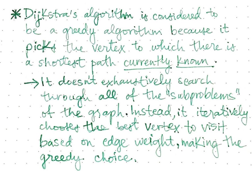
Dijkstra’s algorithm never searches through all of the paths. It isn’t exhaustive in its search; it doesn’t reconsider its choices once it makes them, which means that it won’t search through all of the “subproblems of vertices that it chose not to visit. This can sometimes end up being problematic, because the algorithm could very well not find the most optimal path if it finds a vertex with the shortest path at an early stage, and then proceeds to go down the path of visiting its neighbors.

Okay, so we have divide and conquer algorithms, and we have greedy algorithms. But, let’s get back to the problem at hand: understanding how dynamic programming algorithms compare to these two!

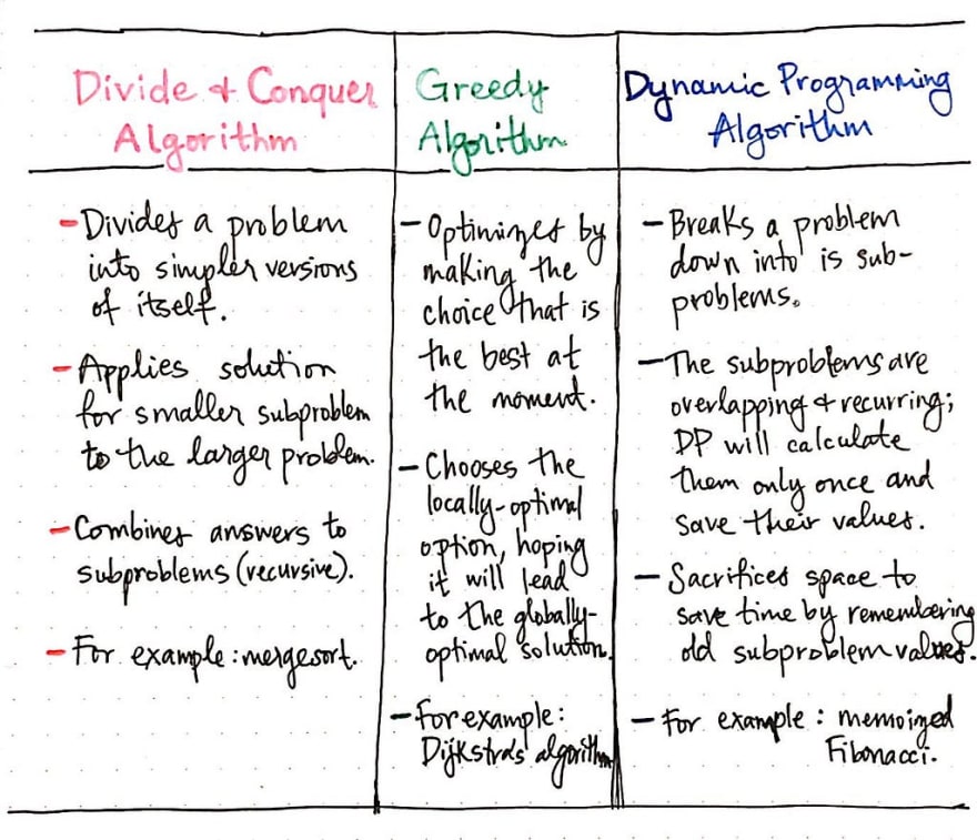
If we compare these three forms of algorithm design to one another, we’ll start to see that there are some obvious similarities (as well as some evident differences) between DP algorithms and its two counterparts.

Looking at the table illustrated above, we can see that DP algorithms are similar to divide and conquer in one obvious way: they both involve breaking down a large problem into smaller, simpler subproblems.

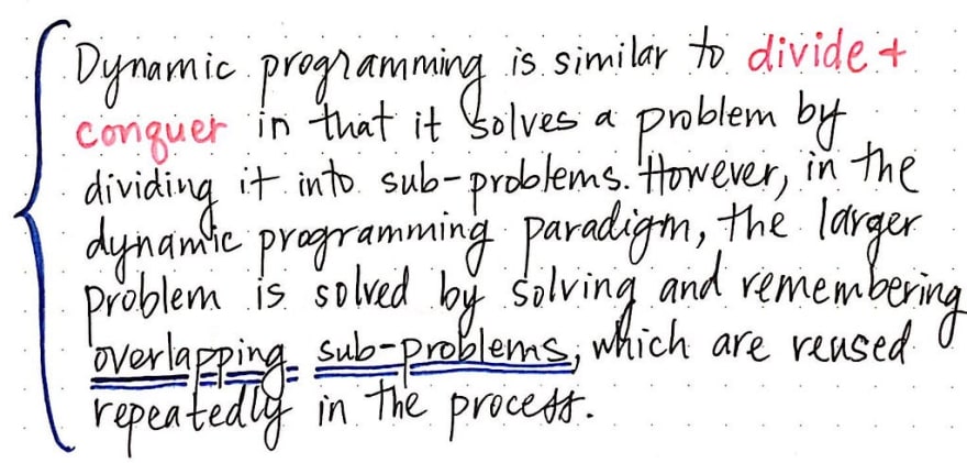
However, we’ll see one major difference between the dynamic programming approach and the divide and conquer one, too. In the DP paradigm, when we break down the larger problem into its smaller parts, those subproblems actually overlap.

Here’s another way to think about it: the subproblems in a dynamic programming algorithm are recurring, and will repeat themselves. In the DP approach, the larger problem is solved by solving and remember overlapping subproblems. In contrast, overlapping subproblems aren’t a requirement for the divide and conquer approach.

So, how does dynamic programming compare to the greedy algorithm paradigm?

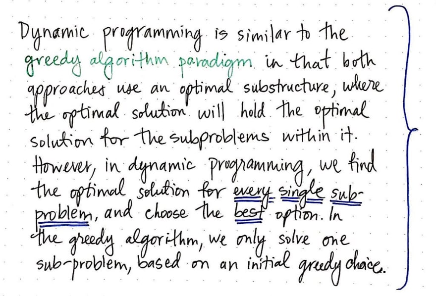
Well, for starters, both approaches have to make choices (ideally the optimal choice) at each stage that the two respective algorithms run. This is often referred to as using an optimal substructure , which refers to the idea that the optimal solution that the algorithm finds will, by proxy, contain the best solution(s) for each of the subproblems inside of it.

However, both of these paradigms approach the problem of “making the best choice possible in starkly different ways.

As we’ve already learned, the greedy algorithm makes an initial greedy choice, and then continues to make the best choice at each stage, setting itself up to solve only one subproblem of the larger, more complex problem. Dynamic programming is very different; the DP paradigm finds the optimal solution for every single subproblem, and chooses the best option from all of the subproblems.

A simpler way to think about how dynamic programming algorithms compare to greedy algorithms is this:

a DP algorithm will exhaustively search through all of the possible subproblems, and then choose the best solution based on that. Greedy algorithms only search through one subproblem, which means they’re less exhaustive searches by definition.

This brings us to an important question: how on earth do dynamic programming algorithms do the work of searching so extensively? How exactly do DP algorithms keep track of all of the overlapping subproblems?

It’s time for us to investigate.

Remember to remember

We already know that dynamic programming is akin to the divide and conquer in that it involves subproblems and breaking down things into easier to calculate pieces. But, we also know that DP algorithms can calculate every single overlapping subproblem that occurs – in other words, if many subproblems exist, it can calculate all of them, and then pick the best one out of the bunch as its final solution.

The trick to calculating all of the solutions to the various subproblems (and then choosing the best one) is remembering previous solutions.

Let’s use a simple example to illustrate what I mean. Imagine we had to solve the problem 5 + 5 + 5 + 5. How would we solve that? Well, we’d just add them up, right? We know that 5 + 5 + 5 + 5 = 20. Done.

But then, what if we just tacked on another 5 at the end of that? 5 + 5 + 5 + 5 + 5 = ?. Mentally, what would we do? Would we add each 5, one after the other, again and again?

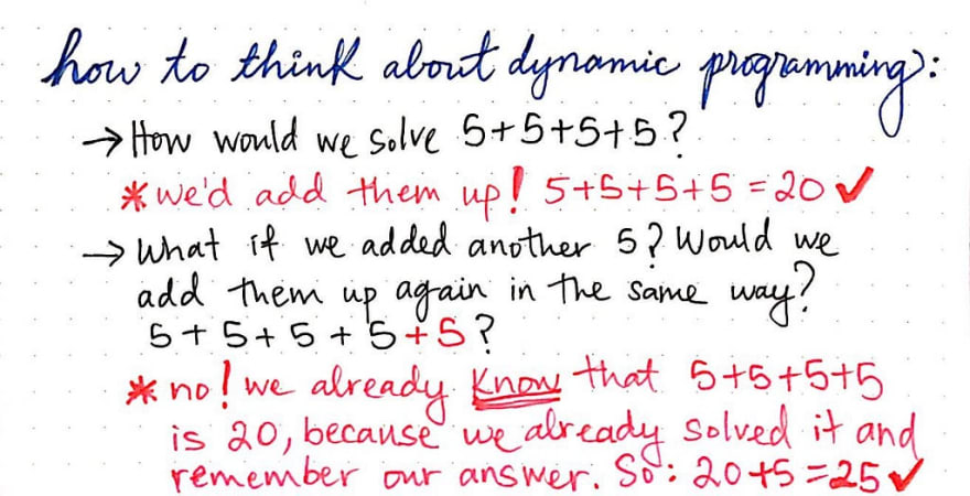
No way! We’d probably just think to ourselves, “Oh, I just did that math. I know it was 20 before, and now there’s another 5, so the answer must be 25!”. We remembered the solution for a problem that we had previously solved before, and used it again when we had to solve a problem that _built upon _it.

Dynamic programming does something similar to what we just mentally worked through in that simple math problem. It remembers the subproblems that it has seen and solved before. When it sees the same subproblem again – which is what we call an overlapping subproblem  – it knows that it doesn’t need to recalculate the work multiple times. It just pulls from the solution that it figured out previously!

The power of dynamic programming is that it allows us to avoid repeating ourselves, and thereby avoid repeating bits of work by remembering partial portions of problems that we have already solved along the way. The ability to not repeat ourselves sounds nice, but it really helps to see it in action. There’s a well-known example that’s used again and again to illustrate how powerful DP algorithms are, and we’re going to look at that very example next. The good news is that we’re already familiar with this famous example: it’s our dear old friend, the Fibonacci sequence!

We’ll recall that the Fibonacci sequence, which is closely tied to the golden ratio, is the sequence of numbers that starts with 0 and 1. In order to derive any number in the Fibonacci sequence, we need to find and sum the two numbers that precede that number.

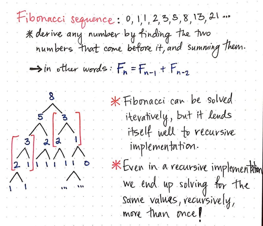
For example, to find the number that comes after 0, 1, 2, 3, 5, we would sum 3 + 5, and know that the next number would be 8. A more abstract way of defining the formula for finding a number in the Fibonacci sequence would be: F[n] = F[n-1] + F[n-2], where n represents the index in an array of Fibonacci numbers. Based on this formula, we also know that Fibonacci can be solved recursively, since we will inevitably find ourselves needing to use recursion to find the previous number in the Fibonacci sequence if we don’t know it already.

However, looking at the example recursive “tree of values that are illustrated above, we’ll notice that we’re repeating ourselves. While recursively solving for the Fibonacci number F[6], or the seventh Fibonacci number, we had to calculate F[5] and F[4]. But then, in order to calculate F[5], we again need to solve for F[4], yet again!

Here’s an example of the same problem of recursive repetition, abstracted out.

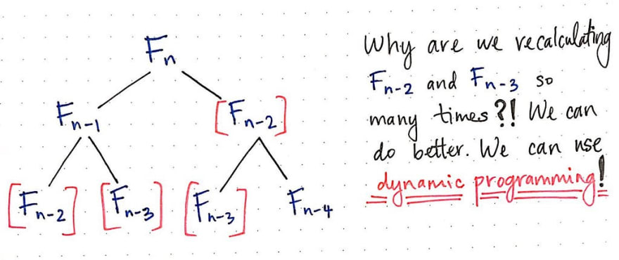
It doesn’t really matter what n is when solving for F[n]; if we use recursion, we’re going to end up having to recalculate portions of the Fibonacci sequence more than once. For example, in the tree above, we are calculating F[n-3] twice, and we’re calculating F[n-2] twice, too. This seems super inefficient, and we should be able to do better.

The good news is: we can! Using dynamic programming, of course.

We know that dynamic programming allows us to remember solutions to problems that we’ve seen and solved before. The Fibonacci example is a prime example of when we would want to remember solutions to Fibonacci numbers that we’ve already solved for! The method for how a DP algorithm remembers problems that it has already solved is known as memoization.

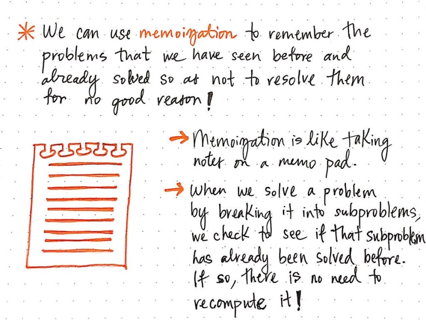
Memoization is a lot like taking notes on a memo pad: when we encounter a problem that seems important (and even if it’s not), we write down the answer to it and note it down, memoizing it. Much like the 5 + 5 + 5 + 5 + 5 problem from earlier, if we run into that same problem later, we don’t need to do the mental math of recomputing all of it. We’ve already solved 80% of the problem because we can reuse our solution from earlier and just build upon it, which is much easier to do than resolving it from the ground up!

Memoization allows us to only run a computation once, and then reuse it later without having to recompute it.

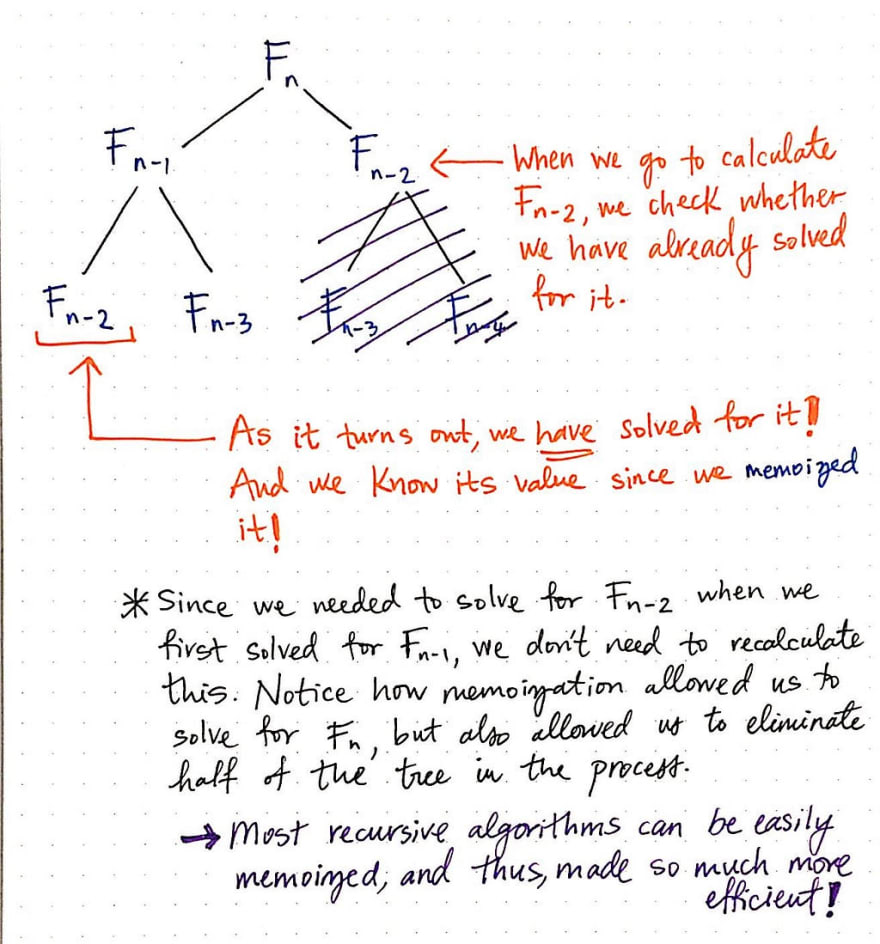
Earlier, before we were using memoization, we needed to calculate multiple subproblems again and again. However, by employing memoization, we can eliminate entire portions of unnecessary work. The illustration shown here exemplifies this.

Now, when solving for F[n], we first calculate F[n-1]. As a part of recursively figuring out the solution to F[n-1], we end up solving for F[n-2] and F[n-3]. Each time that we solve for them for the very first time, we memoize their solutions.

Next, we need to solve for the second part of figuring out F[n]: F[n-2]. When we go to calculate the value of F[n-2], we’ll check to see if we have already solved for it before actually figuring it out. The second time that we see it, we know that we have already solved for it, and we know that we already have its value since we remembered it when we memoized its solution.

Memoization allowed us to eliminate half of this recursive Fibonacci tree, simply because we remembered the solutions to subproblems that we had already seen! As a rule, recursive algorithms, including the Fibonacci algorithm, can be made into dynamic programming algorithms that use memoization for increased optimization and speed.

Okay, so now we know how dynamic programming algorithms manage to find the best, most optimal solution: they solve all the potential subproblems. We also know how they manage to solve all the subproblems: they remember the overlapping solutions, and use memoization to avoid unnecessary computation. But how much more efficient is a dynamic programming algorithm that uses memoization?

Let’s answer that question by looking at the issue of space and time complexity.

Memoize all the things

Without memoization, the runtime complexity of the algorithm to solve for the nth value in the Fibonacci sequence is…not the pretties sight.

For any Fibonacci number at an index of n that we need to solve for, we need to recursively call the same Fibonacci algorithm for the values of n-1 and n-2. We already know some of this math. We know that two quantities have a golden ratio if the ratio between the two quantities is the same as the ratio of the two elements summed when compared to the larger of the two quantities. The combined runtime of these two inner algorithms the time T(n-1) and the time the time T(n-2) ends up amounting to phi (φ or Ï•) raised to the power of whatever n is.

There is also some constant time O(1) that involves summing the numbers and returning the correct value, but that’s negligible. The important thing – the blaring red alarm that should hopefully be going off in our heads – is that there is an exponent involved here! The golden ratio to the nth power as our running time is not good. In fact, it results in exponential running time , or O(2^n)! We always want to avoid that.

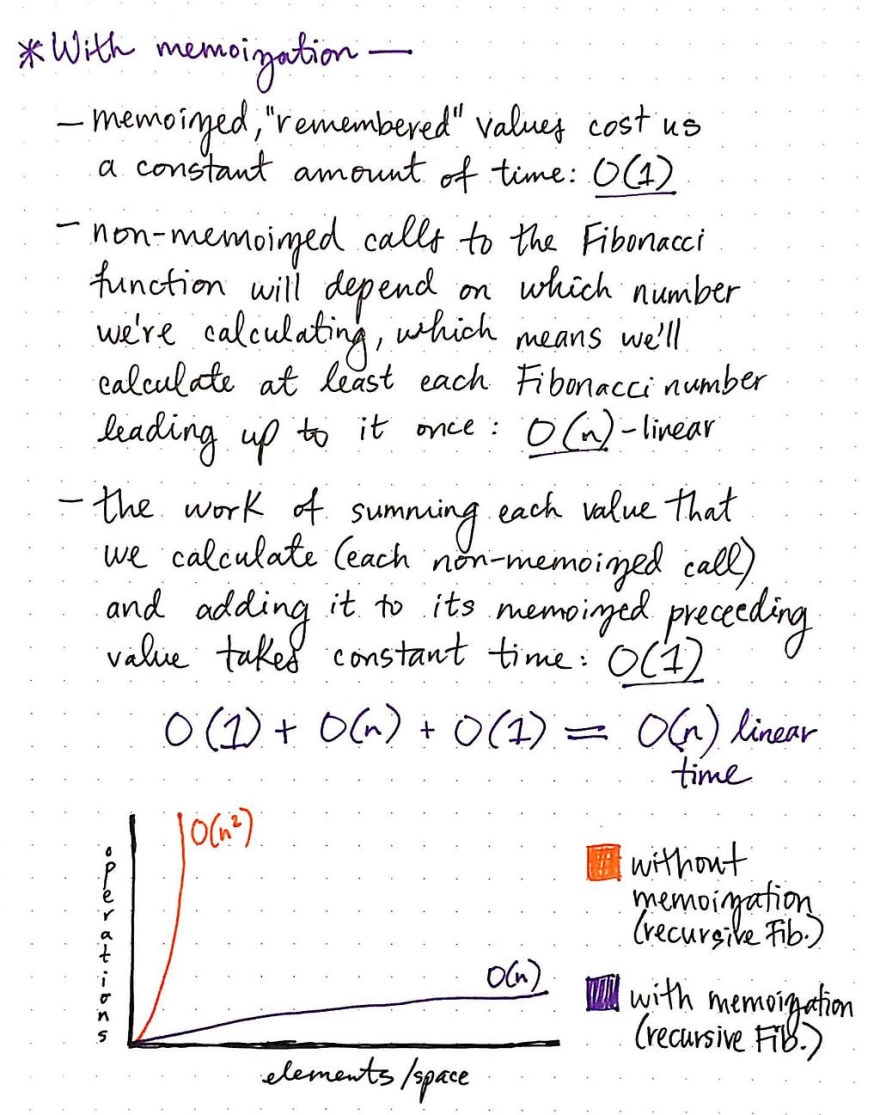
Okay, so without memoization, the recursive form of Fibonacci isn’t too great.

But what about with memoization? Well, the nice thing about “remembered”, memoized values is that they cost us almost no time to actually look up in the dictionary/hash/array where we’d probably store in. In other words, the actual cost of looking up a memoized value costs us O(1), constant  time.

However, the first time that we encounter a subproblem, we still need to to the work of solving it before we can memoize it. The non-memoized calls to the Fibonacci algorithm will depend upon what n is. If we’re looking for the 10th element, it will take us considerable less calls to calculate the Fibonacci sequence than if we were looking for the 100th element. Thus, the work of running the Fibonacci algorithm the first time for each non-memoized element takes linear , O(n) time.

Similar to the non-memoized version of this algorithm, here is also some constant time O(1) that involves summing the numbers and returning the correct value, but that’s negligible. This results in O(n) + O(1) + O(1) runtime, which still amounts to linear , O(n) time.

Linear time is a whole lot better than exponential time! Not bad for a little dynamic programming algorithm, eh?

So how does the memoized version of Fibonacci compare to the non-memoized version when it comes to space?

Given the fact that the memoized version of Fibonacci needs to remember old subproblem solutions, the DP paradigm sacrifices some space in order to save time.

This is part of the tradeoff of using a dynamic programming approach, and depending on how many subproblems we need to solve and how smart we are about the data structure that we use to store those subproblem solutions, sacrificing space for time can often be preferable – particularly if we know we’re going to need to look up many values of Fibonacci, and know that we’ll be reusing our old solutions again and again, later on.

The dynamic programming paradigm is powerful not just for its efficiency, but also for its runtime complexity. However it is worth mentioning that there are two main approaches to DP algorithms; we’ve only really dealt with one in this post, but it’s important to be comfortable in recognizing and using both.

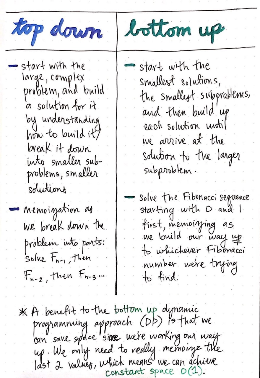
The paradigm of top down dynamic programming is the one that we used in our Fibonacci experiment. In the top down approach, we start with the large, complex problem, and understand how to break it down into smaller subproblems, memoizing the problem into parts.

The alternative to this is the bottom up dynamic programming approach, which starts with the smallest possible subproblems, figures out a solution to them, and then slowly builds itself up to solve the larger, more complicated subproblem.

In the case of solving Fibonacci, the bottom up technique would have involved us solving for the first elements in Fibonacci, and then building our way up to finally arrive at the solution for whatever nth value we were trying to determine to begin with. We would still use memoization to help us store values – we’d just be solving the problem from the “opposite end so to speak. The bottom up approach is probably the one that is more comfortable to most of us when we first learned of Fibonacci. If we think about it, we all start counting Fibonacci with 0, then 1, then 1, then 2, until we count up to the number that we’re looking for.

There is one large benefit to bottom up dynamic programming algorithms, which is this: we only really need to memoize the last two values. Since we know that we’re working our way up – _and not working our way down from the top – we don’t need to work about storing all of the previous values. We really only care about the last two, until we arrive at the value for n. This allows us to eliminate the need for a larger data structure that takes up space for memoized values. Instead, we can just memoize the previous two values, which allows us to achieve **_constant** , or O(1) space.

Dynamic programming, even with all of its idiosyncrasies, isn’t too terrifying once we break it down into its moving parts!

I mentioned earlier that the name “dynamic programming makes it feel more intimidating than it really is. Here’s a funny fact behind DP’s name: it doesn’t really mean anything.

Dynamic programming was invented in the 1940s by Richard Bellman, a computer scientist who was working on mathematical research at a company called RAND at the time. As it turns out, RAND was employed by the US Air Force, which meant that they often had to report to the Secretary of Defense, who was named Charles Erwin Wilson.

In Bellman’s autobiography, Eye of the Hurricane: An Autobiography, he explains how he came up with the name for this paradigm of algorithm design:

[Wilson] actually had a pathological fear and hatred of the word research. I’m not using the term lightly; I’m using it precisely. His face would suffuse, he would turn red, and he would get violent if people used the term research in his presence…Hence, I felt I had to do something to shield Wilson and the Air Force from the fact that I was really doing mathematics inside the RAND Corporation. What title, what name, could I choose? In the first place I was interested in planning, in decision making, in thinking. But planning, is not a good word for various reasons. I decided therefore to use the word “programming”. I wanted to get across the idea that this was dynamic, this was multistage, this was time-varying. I thought, let’s kill two birds with one stone. Let’s take a word that has an absolutely precise meaning, namely dynamic, in the classical physical sense. It also has a very interesting property as an adjective, and that it’s impossible to use the word dynamic in a pejorative sense. Try thinking of some combination that will possibly give it a pejorative meaning. It’s impossible. Thus, I thought dynamic programming was a good name. It was something not even a Congressman could object to. So I used it as an umbrella for my activities.

The moral of the story, if there is such a thing, is that sometimes scarily-named things might actually be named for no other reason than the name sounded good. Therefore, in my opinion, scary-sounding things are nothing to be afraid of! Just be sure not to tell Charles Erwin Wilson that.

Resources

Dynamic programming is a topic that comes up a lot in computer science in the form of difficult problems. Some computer science courses introduce it early on, and then never really come back to address this form of algorithmic design ever again. However, the theory behind dynamic programming comes up again and again, usually in the form of the most complex – and sometimes even unsolvable! – problems. If you’re interested in learning more, here are some great resources to help you get you started.

1. Dynamic Programming – Fibonacci, Shortest Paths, MITOpenCourseWare
2. Algorithms: Memoization and Dynamic Programming, HackerRank
3. Introduction to Dynamic Programming, Hacker Earth
4. Dynamic Programming, Interactive Python
5. Dynamic Programming (Overlapping Subproblems Property), GeeksForGeeks