Big O Notation - explained as easily as possible

Conrad Reeves
Posted on January 19, 2021

— Originally published on that computer scientist. Consider following the original blog for up-to-date articles.
If you want to learn the math involved with the Big O, read Analysing Algorithms: Worst Case Running Time.
Data Structures and Algorithms is about solving problems efficiently. A bad programmer solves their problems inefficiently and a really bad programmer doesn't even know why their solution is inefficient. So, the question is, How do you rank an algorithm's efficiency?
The simple answer to that question is the Big O Notation. How does that work? Let me explain!
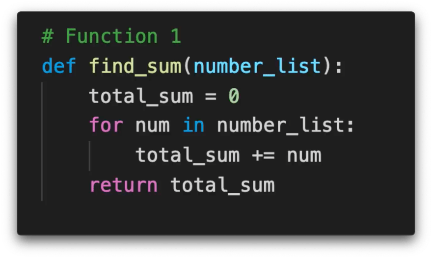
Say you wrote a function which goes through every number in a list and adds it to a total_sum variable.
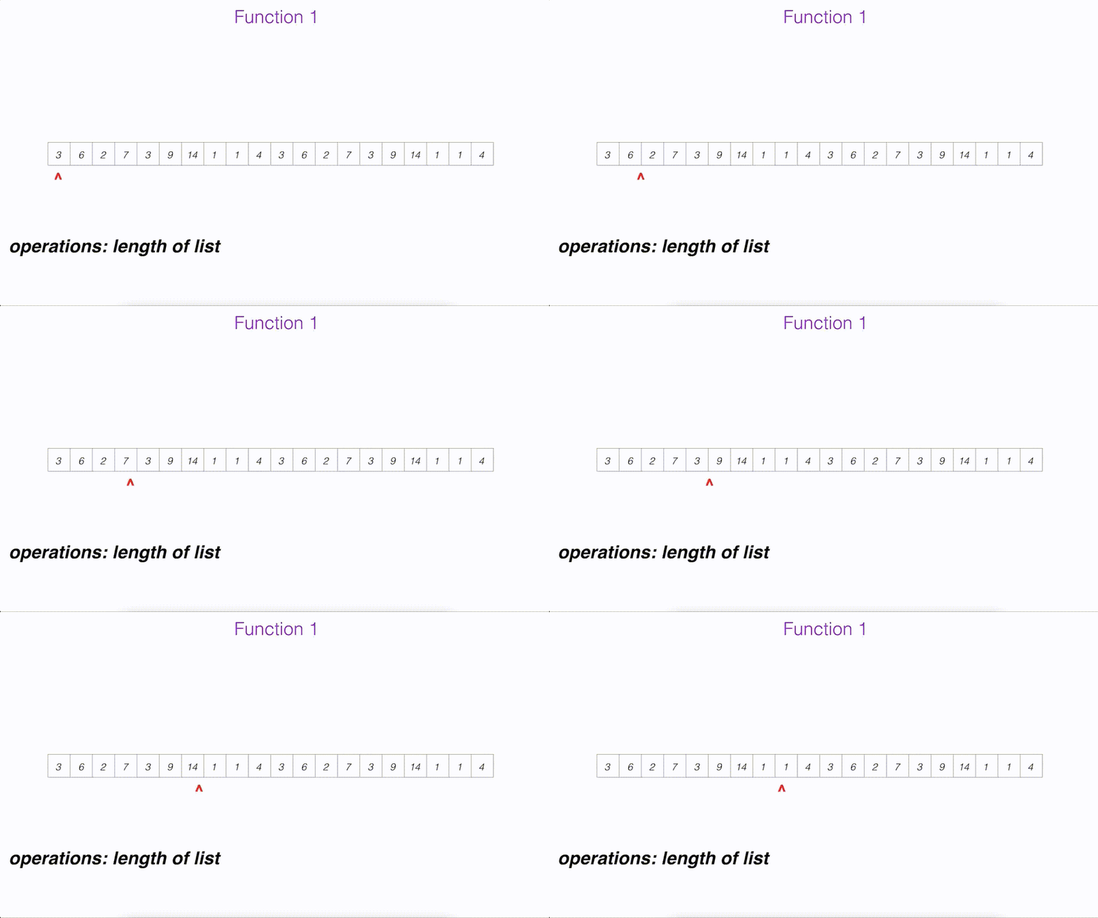
If you consider "addition" to be 1 operation then running this function on a list of 10 numbers will cost 10 operations, running it on a list of 20 numbers costs 20 operations and similarly running it on a list of n numbers costs the length of list (n) operations.
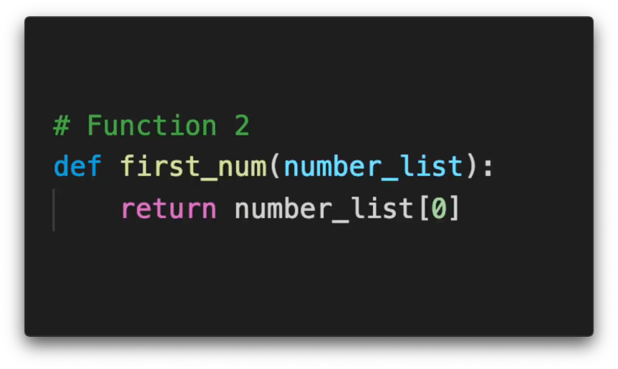
Now let's assume you wrote another function that would return the first number in a list.
Now, no matter how large this list is, this function will never cost more than one operation. Fairly, these two algorithms have different time complexity or relationship between growth of input size and growth of operations executed. We communicate these time complexities using Big O Notation.
Big O Notation is a mathematical notation used to classify algorithms according to how their run time or space requirements grow as the input size grows.
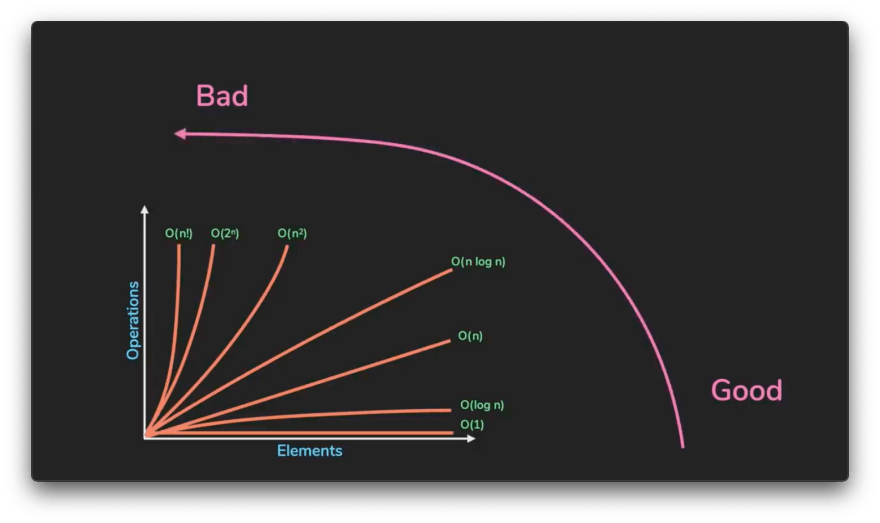
Referring to the complexities as 'n', common complexities (ranked from good to bad) are:
- Constant - O(1)
- Logarithmic O(log n)
- Linear - O(n)
- n log n - O(n log n)
- Quadratic - O(n²)
- Exponential - O(2ⁿ)
- Factorial - O(n!)
Our first algorithm runs in O(n), meaning its operations grew in a linear relationship with the input size - in this case, the amount of numbers in the list. Our second algorithm is not dependent on the input size at all - so it runs in constant time.
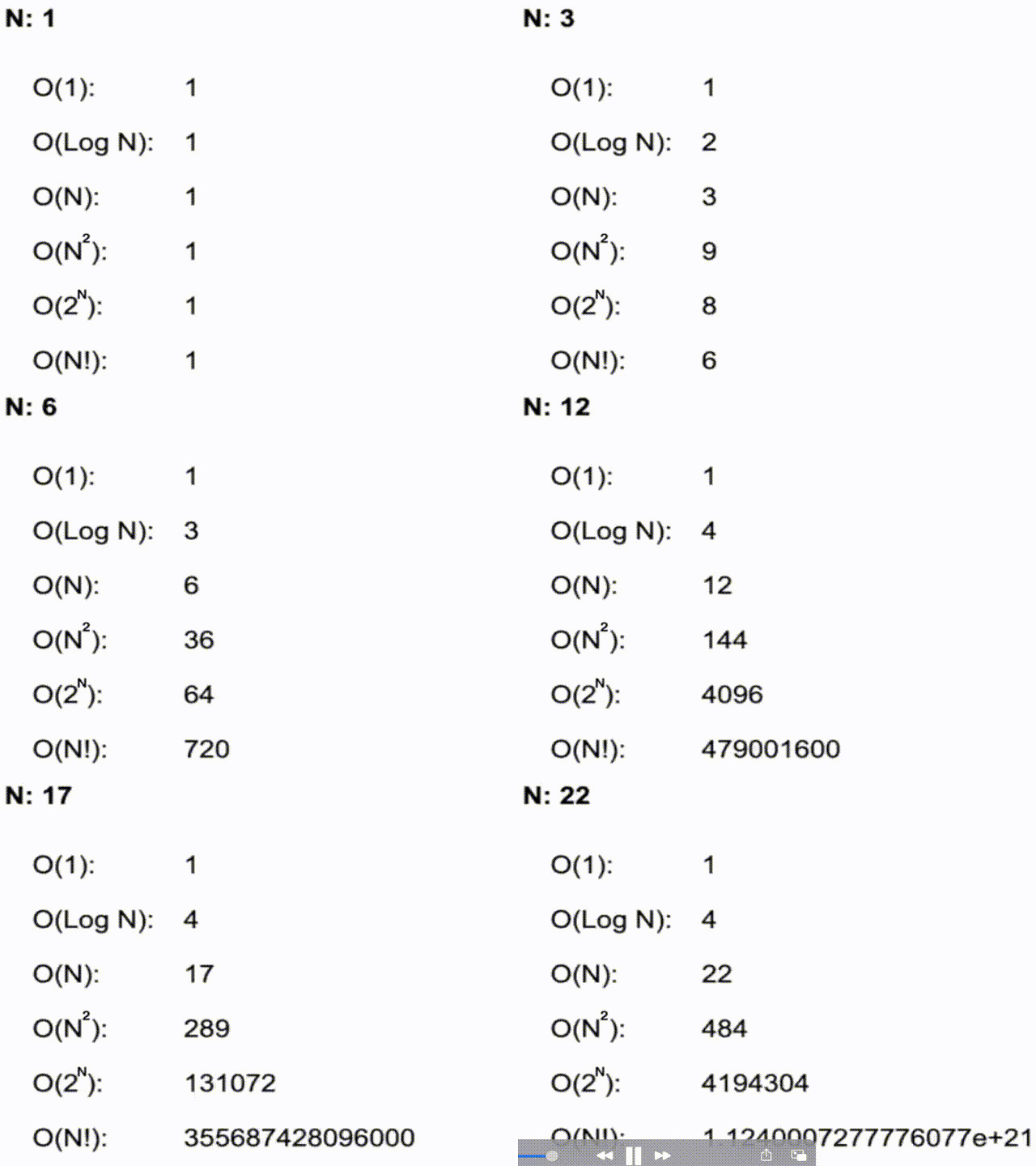
Let's take a look at how many operations a program has to execute in function with an input size of n = 5 vs n = 50.
| n = 5 | n = 50 | |
|---|---|---|
| O(1) | 1 | 1 |
| O(log n) | 4 | 6 |
| O(n) | 5 | 50 |
| O(n log n) | 20 | 300 |
| O(n²) | 25 | 2500 |
| O(2ⁿ) | 32 | 1125899906842624 |
| O(n!) | 120 | 3.0414093e+64 |
It might not matter when the input is small, but this gap gets very dramatic as the input size increases.
If n were 10000, a function that runs in log(n) would only take 14 operations and a function that runs in n! would set your computer on fire!
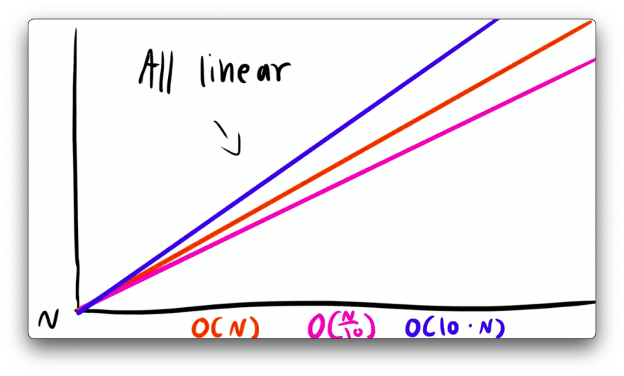
For Big O Notation, we drop constants so O(10.n) and O(n/10) are both equivalent to O(n) because the graph is still linear.
Big O Notation is also used for space complexity, which works the same way - how much space an algorithm uses as n grows or relationship between growth of input size and growth of space needed.
So, yeah! This has been the simplest possible explanation of the Big O Notation from my side and I hope you enjoyed reading this. If you found this information helpful, share it with your friends on different social media platforms and consider clicking those like buttons up there, it really motivates me to write more.
And If you REALLY liked the article, consider buying me a coffee 😊. If you have any suggestions or feedback, feel free to let me know that in the comments.
Happy Programming!

Posted on January 19, 2021
Join Our Newsletter. No Spam, Only the good stuff.
Sign up to receive the latest update from our blog.
